Explicación
A veces nos solicitan generar un archivo Excel, simple, pero otras veces, se necesita contar con el formato indicado, es decir, respetar ceros a la izquierda es un material (MATNR), o formato numerico especial, como separador de miles por coma, y decimal por punto, todo esto se debe manipularlo desde SAP, ABAP, y esta codificación excel, nos sirve para dicho proposito:
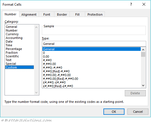
Custom
A custom number format allows you to change and control how your numbers, dates and text are displayed.
When you select "Custom" from the category list you can see all the built-in and custom number formats.
Custom number formats are workbook specific and are saved with your workbook.
Once you delete a custom number format any cells which had it applied, will go back to having the "General" number format.
 |
Formatting Codes - Numbers
| Symbol | Description |
| 0 | Digit placeholder - This symbol pads the number with zeros. This symbol ensures that a specified number of digits appears on each side of the decimal point. For example, if the format is 0.000, the value .987 would be displayed as 0.987. If the format is 0.0000, the value .987 would be displayed as 0.9870. If a number has more digits to the right of the decimal point than the number of 0s specified in the format, the number in the cell is rounded. For example if the format is 0.00, the value .987 would be displayed as 0.99. |
| ? | Digit placeholder - This symbol leaves a space for insignificant zeros to help with alignment. Represents a space on either side of a number. This symbol follows the same rules as the "0" symbol, except that space is left for insignificant zeros on either side of the decimal point. This placeholder aligns numbers on the decimal places. For example 0.34 and 12.45 would line up on the decimal point if both were formatted with 0.?? |
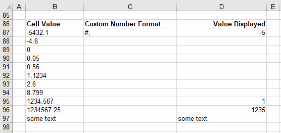
| # | Digit placeholder - This symbol allows separating characters to be added. This symbol follows the same rules as the "0" symbol, except that extra zeros do not appear if the number has fewer digits on either side of the decimal point. This symbol shows Excel where to display commas or other separating symbols. The format #,### for example displays a comma after every third digit to the left of the decimal place. |
| . | Decimal point placeholder - This symbol determines how many digits (0 or #) appear to the right or left of the decimal point. If the format contains only #s to the left of the decimal point, numbers smaller than 1 will start with a decimal point. To avoid this, use 0 as the first digit placeholder to the left of the decimal point instead of #. If you want Excel to include commas and display at least one digit to the left of the decimal point in all cases specify the format as #,##0. |
| % | Percentage Indicator - This symbol multiples the value by 100 and a percentage sign is added to the end. |
| / | Fraction format character - This symbol displays the fractional part of a number in a nondecimal format. The number of digit placeholders that surround this character determines the accuracy of the display. For example, the decimal fraction 0.269 when formatted as #?/? is displayed as 1/4 but when formatted with #???/??? is displayed as 46/171 |
| , (comma) | Thousand separator - A comma followed by a placeholder scales the number by 1000. If the format contains a comma surrounded by #s, os or ?s Excel uses commas to separate hundreds from thousands, thousands from millions etc. In addition the comma acts as a rounding and scaling agent. Use one comma at the end of a format to tell Excel to round a number and display is in thousands; two commas tell Excel to round to the nearest million. For example the format #,###,###, rounds 4567890 to 4,568 (thousands) and the format #,###,###,, rounds the same number to 5 (millions). |
Formatting Codes - Text
| E+ E- e+ e- | Scientific format characters. If a format contains one 0 or # to the right of an E-, E+, e- or e+, the number is displayed in scientific notation and the characters E or e are inserted into the displayed number. The number of 0s or #s to the right of the E or e determines the minimum number of digits in the exponent. Use E- or e- to place a negative sign by negative exponents and use E+ or e+ to place a positive sign by positive exponents. |
| $ - + / ( ) space | Standard formatting characters which are displayed in your format. |
| \ character | Special characters. This displays the specific character. Typing ! ^ & ` ~ { } = < > automatically places a backslash in front of the character. Precede each character you want to display in the cell (except for : $ - + / ( ) and space) with a backslash. The backslash is not displayed. The backslash can be used insert single characters. To insert several characters use the quotation mark "". |
| _ (underscore) | This code skips the width of the next character. Represents a space that is the same width as the character that follows in the code string. This code is commonly used as "_)" (without the quotation marks) top leave space for a closing parenthesis in a positive number format when a negative number format includes parentheses. This allows the values to line up at the decimal point. |
| "Text" | Literal character string - Displays the text string within the quotation marks. |
| * | Repetition initiator - This is used to pad the cell with the character immediately after it. Fills the empty space by repeating a character that you specify. Repeats the next character to fill the column width. Only one asterisk per section is allowed. |
| @ | Text placeholder. |
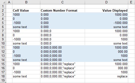
Default Sections - Positive; Negative; Zero; Text
Custom number formats can contain up to four sections separated by semicolons.
Text will always have the "General" number format applied unless there are four sections.
Positive - If there is only one section provided then this format is applied to all positive, negative and zero values.
Negative - If two sections are provided, the first is applied to all positive and zero values. The second is applied to all negative values.
Zero Values - If three sections are provided, the first is applied to all positive values, the second to all negative values and the third to all zero values.
Text - If four sections are provided then the last section will be applied to any text values.
 |
Adding Colours
It is possible to automatically change the colour of the value (or text) depending on the values (or characters) that are in the cells.
You can display different values in different colours.
This allows you to emphasis particular values in the worksheet.
#,###.00_);[Red](#,###.00);0.00;[Green]"The department is"@
Note that any colours that you specify with a number format will take precedence over any manual formatting applied.
It is not possible to display different parts of the text in different colours using this method.
To define a colour place it in square brackets at the start of the section.
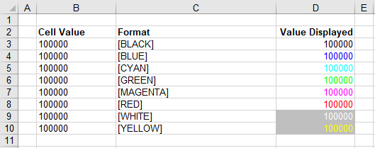 |
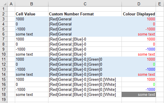
Each of the four categories (positive, negative, zero, text) can have its own colour associated with it.
When you just enter a colour with no explicit number format, "General" will be applied automatically.
[Red] will make everything the colour red, positive, negative, zero and text.
[Red];[Blue]-0 will make everything the colour red (inc zero and text), except for negative numbers which will be blue.
[Red];[Blue]-0;[Green]0 will make positive numbers red; negative numbers will be blue; zero values will be green.
[Red];[Blue]-0;[Green]0;[White] will make positive numbers red, negative numbers will be blue, zero values will be green; text will be white.
 |
Custom Sections - Adding A Condition
It is possible for a number format to contain custom conditions.
These conditions can contain one of the comparison operators ( < > = <= >= <> ).
Each section can contain a numerical condition as well as a custom colour.
[<3000][RED]0;0
[<20][RED]0;[>40][GREEN]0
When you use a custom condition in your number format the Positive, Negative, Zero convention No Longer Applies.
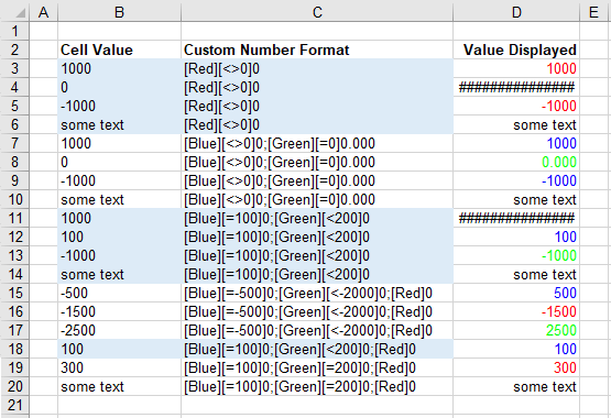 |
Section1 - Lets assume there is only one section provided and this section contains a condition.
All the values that meet this first condition will have this format applied to them. Example Row 3.
If a value does not match this first condition then no number format will be applied. Example Row 4.
Section2 - Lets assume there are only two sections provided and they both contain conditions.
All the values that meet the first condition will have the first format applied to them. Example Row 6.
All the values that meet the second condition will have the second format applied to them. Example Row 7.
If a value meets both the first and the second condition then the first format will be applied. Example Row 10.
If a value does not match the first or the second condition then no number format will be applied. Example Row 9.
Section3 - Lets assume there are only three sections provided and the first two contain conditions.
All the values that meet the first condition will have the first format applied to them. Example Row 12.
All the values that meet the second condition will have the second format applied to them. Example Row 14
If a value meets both the first and the second condition then the first format will be applied.
If a value does not match the first or the second condition then the third format will be applied. Example Row 16.
Text - If four sections are provided then the last section will override any text values with the format provided in the fourth section.
Creating New Formats
To create a custom number format you can either type it directly into the Type textbox or you can edit an existing format.
To create a custom format select the cells, and select the custom category.
Type in the appropriate codes to define the format you want.
You can use the "Delete" button to remove a custom number format.
You cannot remove any of the built-in number formats.
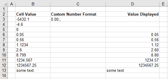
Example 1 - Hiding Negative and Zero Values
Worksheets can often display erroneous zero values particularly when formulas are referencing blank cells.
Number Format : 0.00;;
It is also possible to hide just zero values by using the (Options, Advanced)(Display - Worksheet group).
 |
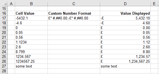
Example 2 - Currency Symbol on LHS
If you want to have your currency symbols appearing on the left of the cell rather than to the left of the value, just include an asterisk and a space after the currency symbol when entering the custom number format.
The asterisk means to repeat the character and in this case it's a space to fill the width of the column.
Number Format : £* #,##0.00;-£* #,##0.00
 |
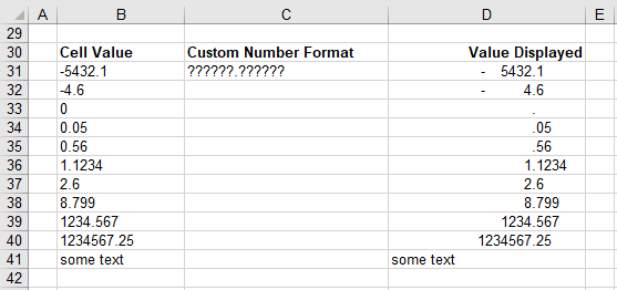
Example 3 - Align Decimal Points
If you want to align all the decimal points.
Just make sure you include enough question marks on either side of the decimal place to accommodate all your digits.
Number Format : ??????.??????
 |
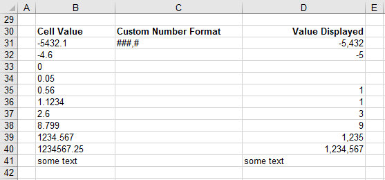
Example 4 - Rounded to Whole Numbers
If you want to have your numbers rounded up to whole numbers.
Any positive numbers are rounded up.
Any negative numbers are rounded down.
Number Format : ###,#
 |
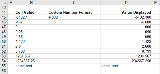
Example 5 - Display 3 Decimal Places
If you want to have your numbers rounded to 3 decimal places.
Number Format : #.000
 |
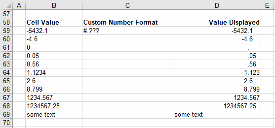
Example 6 - Display 3 Decimal Places without Insignificant Zeros
If you want to have your numbers rounded to 3 decimal places with any insignificant zeros removed.
Number Format : #.???
 |
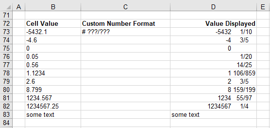
Example 7 - Whole Number and Fraction
If you want to have the numbers displayed as a whole number and a corresponding fraction.
Number Format : # ???/???
 |
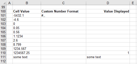
Example 8 - Display in Thousands
To display numbers in thousands create a number format that ends with one comma.
Number Format : #,
 |
To display numbers in millions create a number format that ends with two commas.
Number Format : #,,
 |
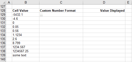
Example 9 - Hide Everything
You can hide numerical data in cells with the null format.
Just apply a different format in order to view the values.
Number Format : ;;; (semi-colons)
 |
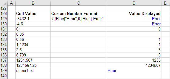
Example 10 - Negative or Text As Blue Error
To display any negative numbers or text with blue Error text
Number Format : ?;[Blue]"Error";0;[Blue]"Error"
 |
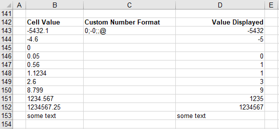
Example 11 - Hiding Zeros and Decimal Places
If you want to hide all zero values and any decimal places.
Number Format : 0;-0;;@
 |
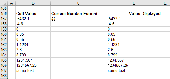
Example 12 - Text and Left Aligned
If you want to have all the numbers converted to text and left aligned.
This is the custom number format used when you choose the standard "text" number format.
Number Format : @
 |
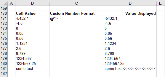
Example 13 - Text and Left Aligned with Padding
If you want to have all the numbers converted to text, left aligned with text values padded.
Number Format : @*>
 |
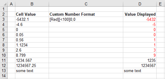
Example 14 - Less Than 100 In Red
To display all numbers that are less than 100 in Red (including positive, negative and zero).
Number Format : [Red][<100]0;0
Positive numbers greater than 100 do not meet the condition in the first section.
There is another section so everything else has this format applied to it.
Including the positive numbers that are greater than 100, rows 151 and 152.
There is no custom format specified for text values so these are displayed using the default format which is black text.
 |
Remove Percentage Symbols - (Ctrl + J)
If you want to link to a cell formatted as a percentage, but not display the percentage symbol.
SS - cell with 0.12, formatted as a percentage
linked to cell below
Enter 0, press (Ctrl + J) to insert a carriage return and then enter the % symbol on the line below.
Wrap the cell - Alignment tab, wrap text
Important
Using a lot of custom number formats in a single workbook will use up a lot of memory.
Every time you edit a custom number format it will be added to the list. You should delete any custom number formats that you are not using.
Source (Fuente):
https://bettersolutions.com/excel/formatting/number-tab-custom-format.htm
Comentarios
Publicar un comentario